Quickstart#
This guide will show how to search, download and plot basic STIX observations for more detailed information on the instrument and observations please see STIX.
Installation#
pip install stixpy
Quicklook Search and Download#
Data search download is built on Sunpy’s Fido and provides easy search and download of data. To search for some quicklook X-ray light curve data run the following commands
from sunpy.net import Fido, attrs as a
from stixpy.net.client import STIXClient  # This registers the STIX client with Fido

ql_query = Fido.search(a.Time('2020-06-05', '2020-06-07'), a.Instrument.stix,
                    a.stix.DataProduct.ql_lightcurve)
This should return a list of data files similar to this.
ql_query
<sunpy.net.fido_factory.UnifiedResponse object at 0x1133e0e10>
Results from 1 Provider:

3 Results from the STIXClient:
       Start Time               End Time        Instrument Level DataType  DataProduct  Ver Request ID
----------------------- ----------------------- ---------- ----- -------- ------------- --- ----------
2020-06-05 00:00:00.000 2020-06-05 23:59:59.999       STIX    L1       QL ql-lightcurve V01          -
2020-06-06 00:00:00.000 2020-06-06 23:59:59.999       STIX    L1       QL ql-lightcurve V01          -
2020-06-07 00:00:00.000 2020-06-07 23:59:59.999       STIX    L1       QL ql-lightcurve V01          -
Downloading the data is then a simple as fetching the data.
ql_files = Fido.fetch(ql_query)
Quicklook Plots#
One we have the data downloaded we can create timeseries from the fits files, following on from the above code.
from datetime import datetime
from sunpy.timeseries import TimeSeries
from stixpy.timeseries import quicklook # This registers the STIX timeseries with sunpy
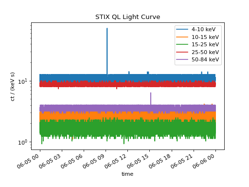
ql_lightcurves = TimeSeries(ql_files)
ql_lightcurves[0].peek()
(Source code, png, hires.png, pdf)

The three separate time series can easily be concatenated to plot the entire time range
combined_ts = ql_lightcurves[0]
for lc in ql_lightcurves[1:]:
    combined_ts = combined_ts.concatenate(lc)

combined_ts.peek()
(Source code, png, hires.png, pdf)
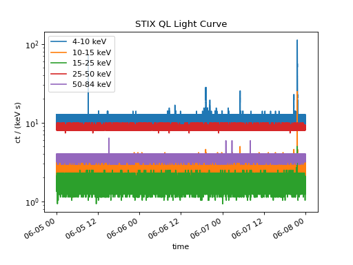
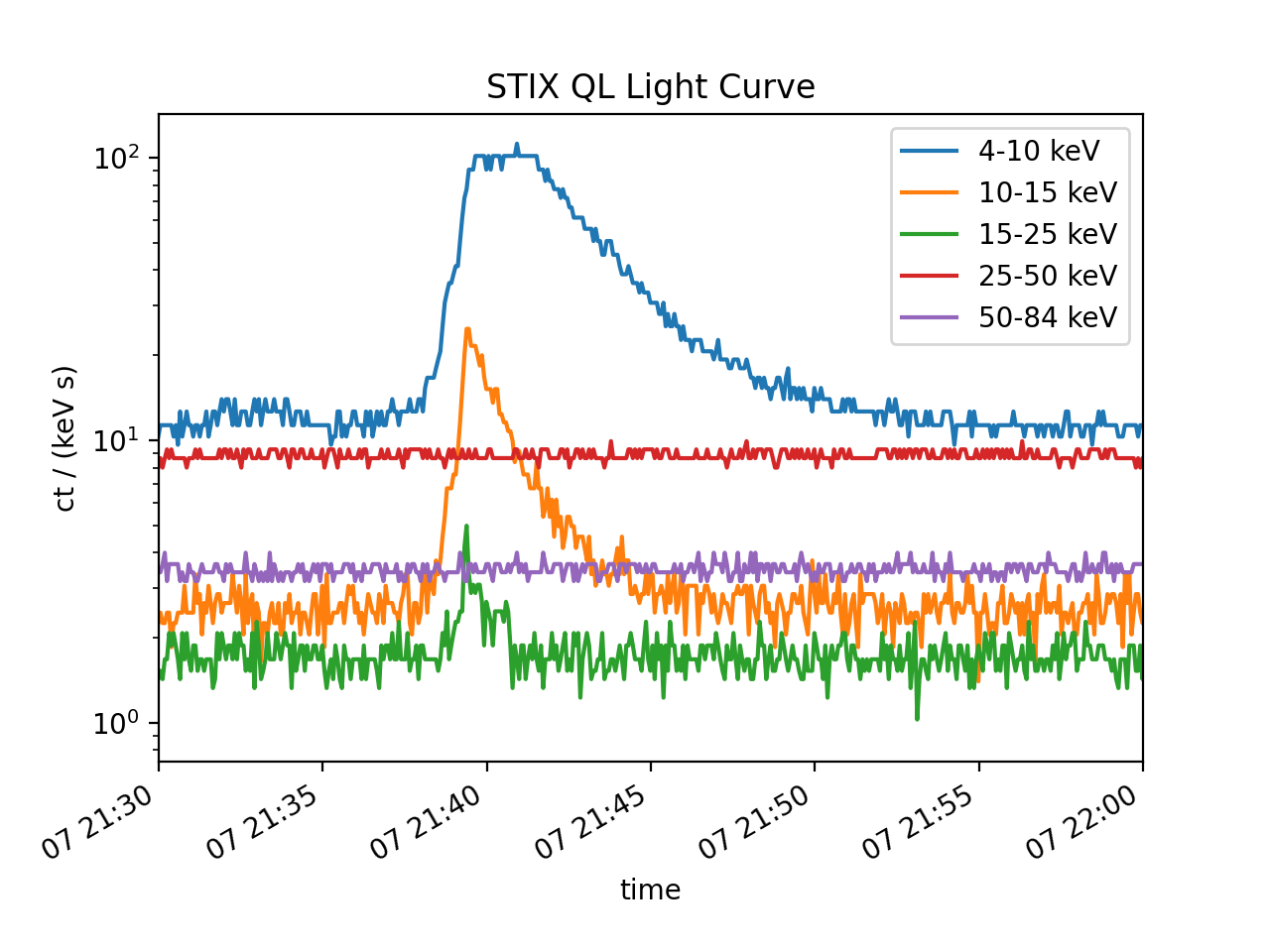
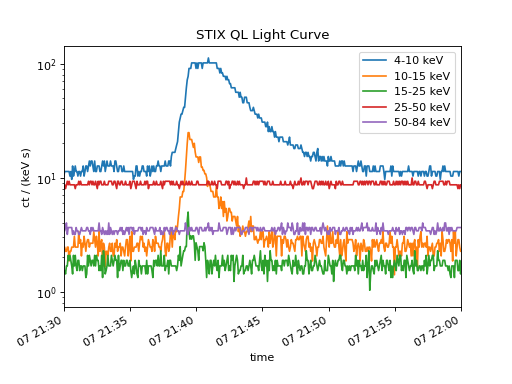
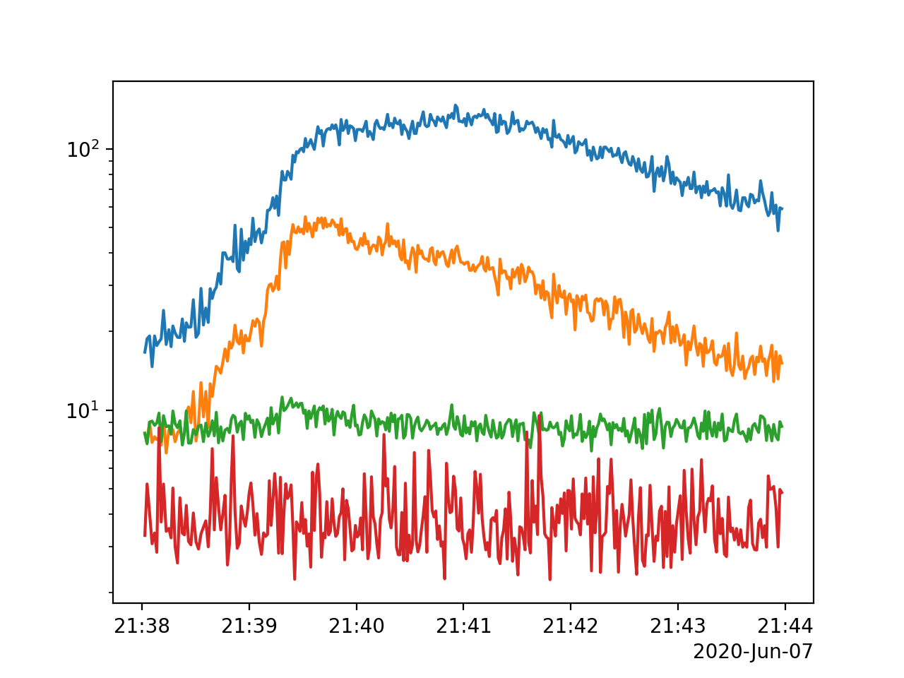
There is a larger flare toward the end of the time range lets zoom in on this region from 21:30 to 22:00 on 2020-06-07.
combined_ts.plot()
plt.xlim(datetime(2020, 6, 7, 21, 30), datetime(2020, 6, 7, 22, 0))
(Source code, png, hires.png, pdf)
Science Data Search and Download#
No we’ve located a flare of interest lets search for some full resolution science data, we can use the same approach for quicklook data above but change the query to search a narrower time window and search only for science data.
sci_query = Fido.search(a.Time('2020-06-07T21:30', '2020-06-07T22:00'), a.Instrument.stix,
                        a.stix.DataType.sci)
sci_query['stix'].filter_for_latest_version() # only keep latest versions
This should return a list of data files similar to this.
sci_query
<sunpy.net.fido_factory.UnifiedResponse object at 0x11385f198>
Results from 1 Provider:

8 Results from the STIXClient:
       Start Time               End Time        Instrument Level DataType  DataProduct  Ver Request ID
----------------------- ----------------------- ---------- ----- -------- ------------- --- ----------
2020-06-07 21:34:10.000 2020-06-07 21:37:09.000       STIX    L1      SCI  sci-xray-cpd V01 1178427920
2020-06-07 21:34:10.000 2020-06-07 21:52:08.000       STIX    L1      SCI  sci-xray-cpd V01 1178427921
2020-06-07 21:35:22.000 2020-06-07 21:45:23.000       STIX    L1      SCI  sci-xray-cpd V01 1178428176
2020-06-07 21:37:09.000 2020-06-07 21:52:08.000       STIX    L1      SCI  sci-xray-cpd V01 1178428688
2020-06-07 21:37:59.000 2020-06-07 21:40:39.000       STIX    L1      SCI  sci-xray-cpd V01 1178428944
2020-06-07 21:39:12.000 2020-06-07 21:39:28.000       STIX    L1      SCI  sci-xray-cpd V01 1178429200
2020-06-07 21:37:59.000 2020-06-07 21:41:59.000       STIX    L1      SCI sci-xray-spec V01 1178428992
2020-06-07 21:37:59.000 2020-06-07 21:43:59.000       STIX    L1      SCI sci-xray-spec V01 1178428992
Lets download a spectrogram (spec) and some compressed pixel data (cpd) that cover a similar time range.
Note
The order the downloaded files are returned may vary so bear this in mind, hence the use of sort.
sci_files = Fido.fetch(sci_query[0][[4,-1]])
sci_files = sorted(sci_files)
Now lets create a spectrogram, similar to Sunpy Map and TimeSeries stixpy Procduct can take a number of input types and will return the correct product type. In this case we are providing the path to to spectrogram fits file.
from stixpy.product import Product
spec = Product(sci_files[1])
spec
Spectrogram   <sunpy.time.timerange.TimeRange object at 0x1229d04a8>
Start: 2020-06-07 21:37:59
End:   2020-06-07 21:43:59
Center:2020-06-07 21:40:59
Duration:0.004170138888888952 days or
       0.10008333333333486 hours or
       6.005000000000091 minutes or
       360.30000000000547 seconds
DetectorMasks
[0]: [0,1,2,3,4,5,6,7,_,_,10,11,12,13,14,15,16,17,18,19,20,21,22,23,24,25,26,27,28,29,30,31]

PixelMasks
[0...339]: [['1' '1' '1' '1' '1' '1' '1' '1' '1' '1' '1' '1']]

EnergyEdgeMasks
[0]: [0,1,2,3,4,5,6,7,8,9,10,11,12,13,14,15,16,17,18,19,20,21,22,23,24,25,26,27,28,29,30,31]
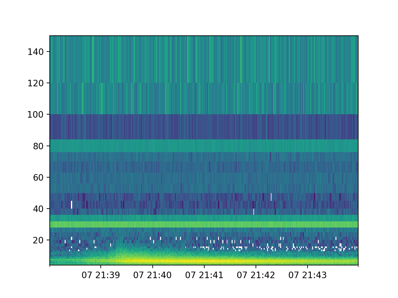
A spectrogram plot can be obtained by call the plot_spectrogram method.
spec.plot_spectrogram()
(Source code, png, hires.png, pdf)
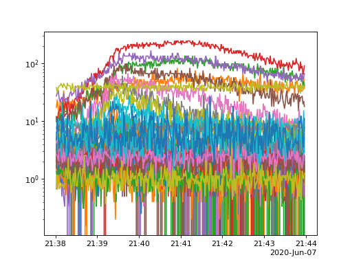
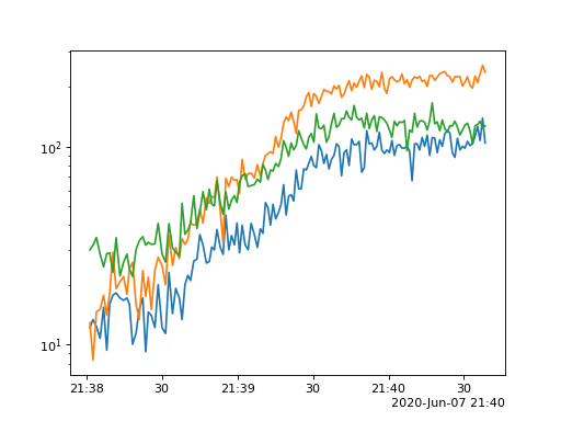
A timeseires can also be created by calling plot_timeseries, by default this will sum all pixel and detectors present
in the data.
spec.plot_timeseries()
(Source code, png, hires.png, pdf)

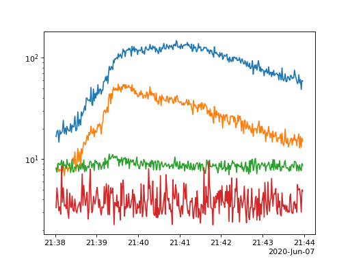
By default the plot methods plot all data present however it is easy to sum over time and or energy
spec.plot_timeseries(energy_indices=[[1, 4], [4, 10],[10, 20], [20, 30]])
(Source code, png, hires.png, pdf)

Now let look at the pixel data, the data can be loaded just same as the spectrogram.
cpd = Product(sci_files[0])
cpd
CompressedPixelData   <sunpy.time.timerange.TimeRange object at 0x1150dc160>
Start: 2020-06-07 21:37:59
End:   2020-06-07 21:40:39
Center:2020-06-07 21:39:19
Duration:0.0018576388888887907 days or
       0.04458333333333098 hours or
       2.6749999999998586 minutes or
       160.49999999999153 seconds
DetectorMasks
[0...146]: [0,1,2,3,4,5,6,7,8,9,10,11,12,13,14,15,16,17,18,19,20,21,22,23,24,25,26,27,28,29,30,31]

PixelMasks
[0...146]: [['1' '1' '1' '1' '1' '1' '1' '1' '0' '0' '0' '0']]

EnergyEdgeMasks
[0]: [_,_,2,3,4,_,_,_,_,_,_,_,_,_,_,_,_,_,_,_,_,_,_,_,_,_,_,_,_,_,_,_]
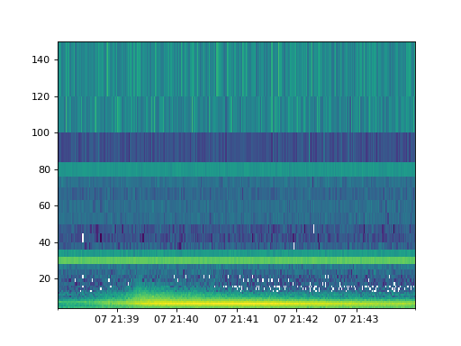
Pixel data supports the same plot methods as spectrogram but notice the plots only contain 3 energy channels as the data file only contains 3 energy channels.
cpd.plot_spectrogram()
(Source code, png, hires.png, pdf)

cpd.plot_timeseries()
(Source code, png, hires.png, pdf)

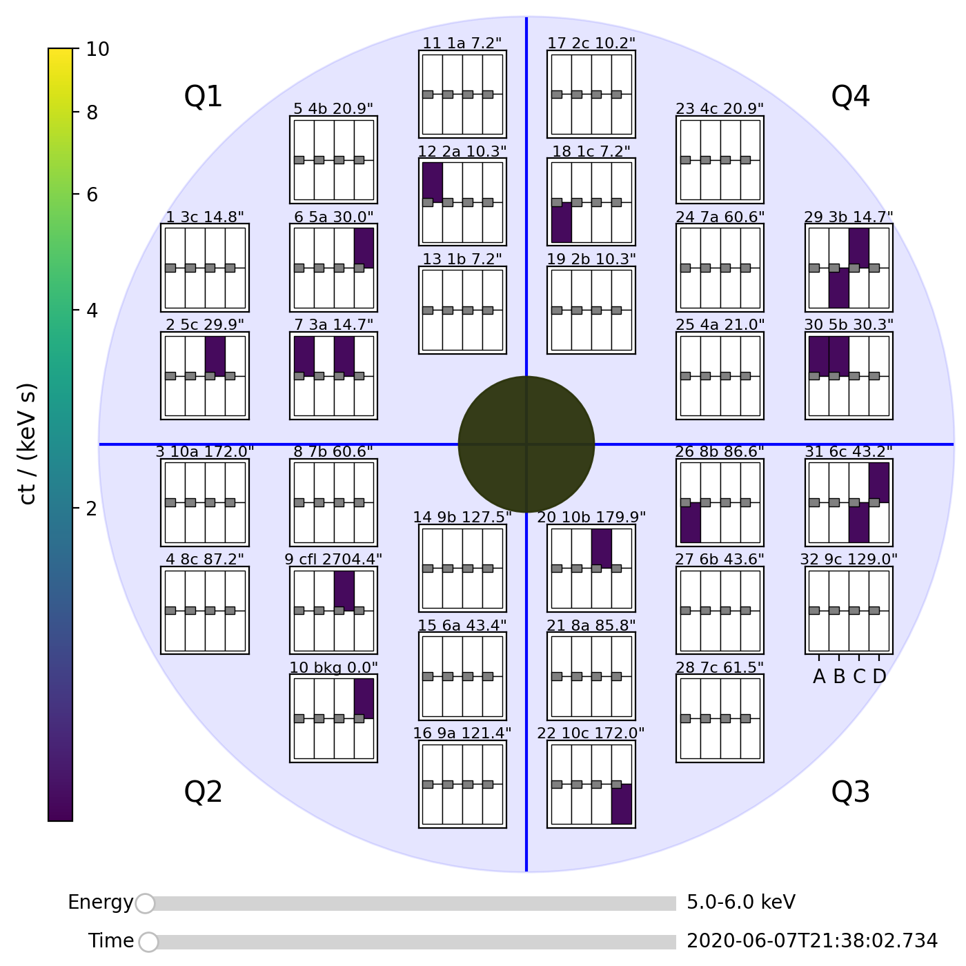
and one additional method plot_pixels.
cpd.plot_pixels()
(Source code, png, hires.png, pdf)
